Have you ever wondered how to change the legend text in Excel charts?
When you create a graph in Excel, the legend usually displays the names of the columns from your data table.
But what if you want the legend text to be different from your table columns?
Of course, you can change the column name to alter the legend text.
But what if you want the legend text to have a different name than the table columns?
Is that possible in Excel?
Yes, it is!
In this article, you will learn how to change legend text in Excel, step-by-step.
Also read: (opens in new tab)
How to Switch Back to the Old Layout in Google Docs
Smooth Scrolling Google Sheets
How to Print Labels From Google Sheets for Free
Google Doc Cursor Parking Lot
How to Change Legend Text in Excel
Step 1: Click on the chart to select it
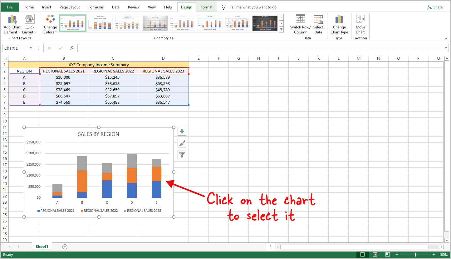
First, open the Excel file and select the sheet containing the chart and table.
Once you have opened the sheet, click on the chart to select it.
Step 2: Select the “Design” option from the top menu
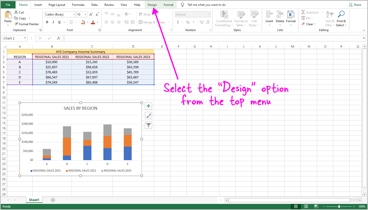
After clicking on the chart, select the “Design” option from the top menu.
Step 3: Click on “Select Data”
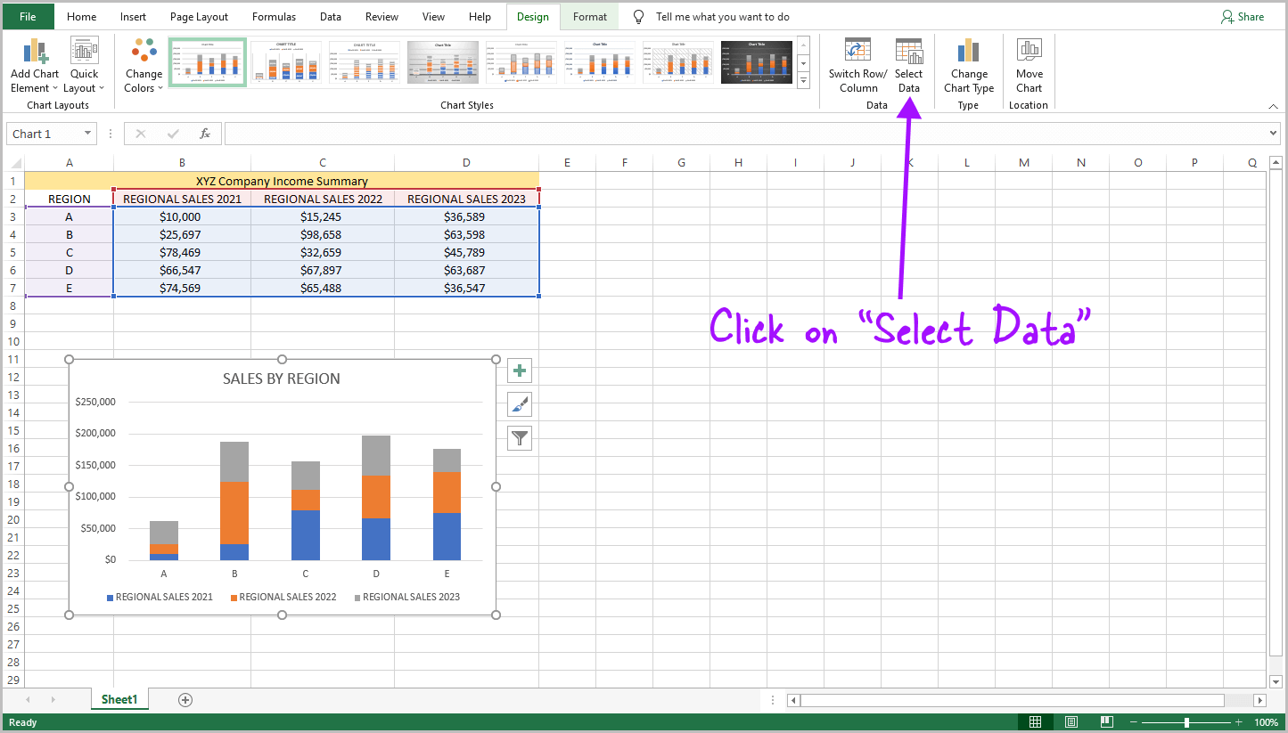
From the “Design” menu, select “Select Data”.
Step 4: Select a legend entry and click on “Edit”
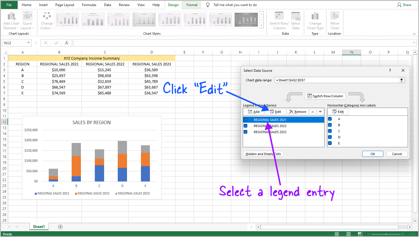
You will now see a pop-up window titled “Select Data Source”.
In the “Legend Entries (Series)” box, you will find all the legend entries.
Click on the entry that you want to modify.
After selecting the entry, ensure that it is highlighted in blue, indicating that you have correctly selected it.
Next, click on the “Edit” button inside the “Legend Entries (Series)” box.
Step 5: Enter the new name in the “Series name:” area and click “OK”
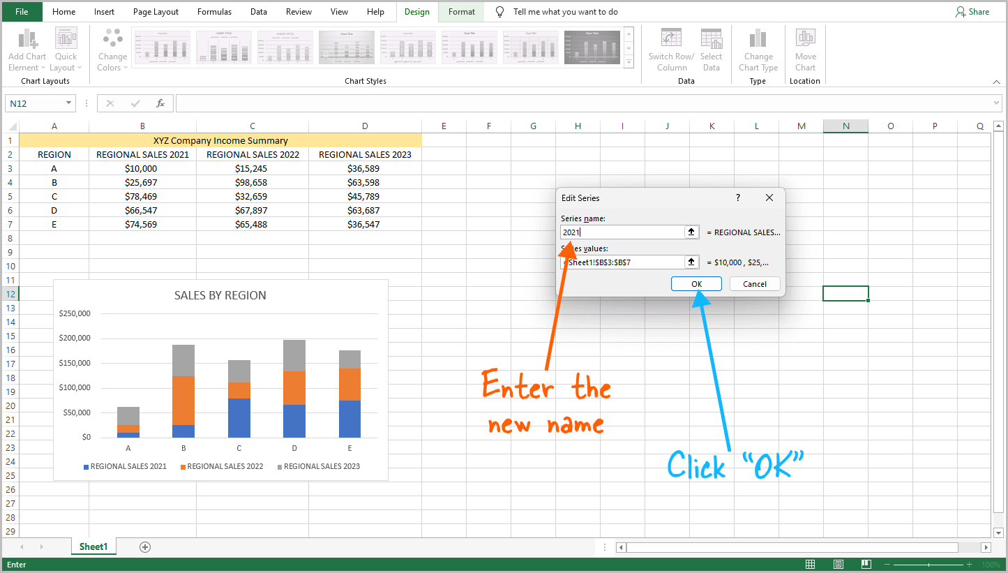
A small pop-up window titled “Edit Series” will appear.
Delete the text in the “Series name:” field and enter the new name for the legend.
Click “OK” to close the pop-up.
Step 6: Repeat steps 4-5 for the other legend entries
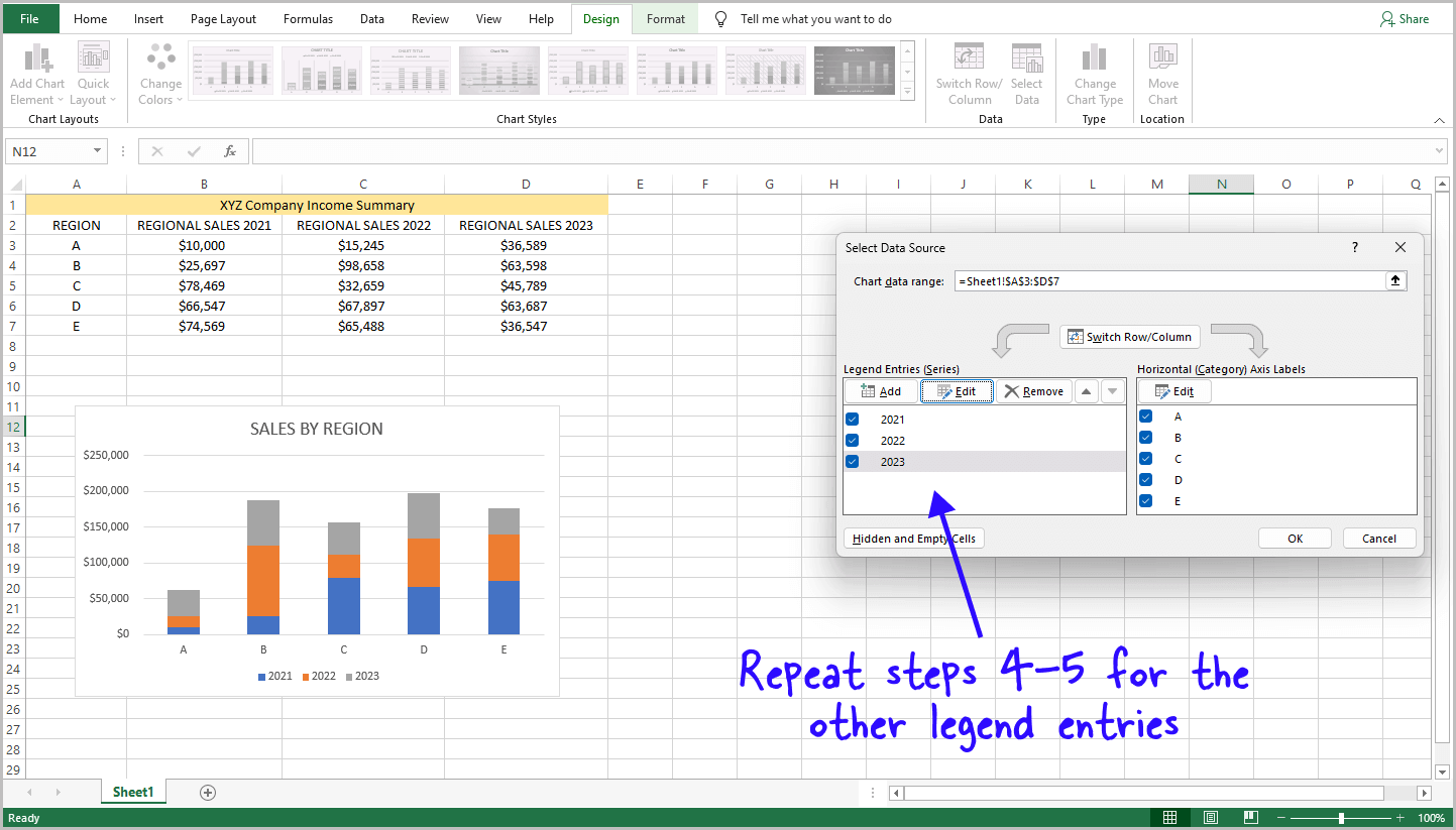
Now, repeat step 4 and step 5 to change the names of the other legend entries.
Once you have updated all the names, proceed to the next step.
Step 7: Click “OK” on the “Select Data Source” window to confirm the changes
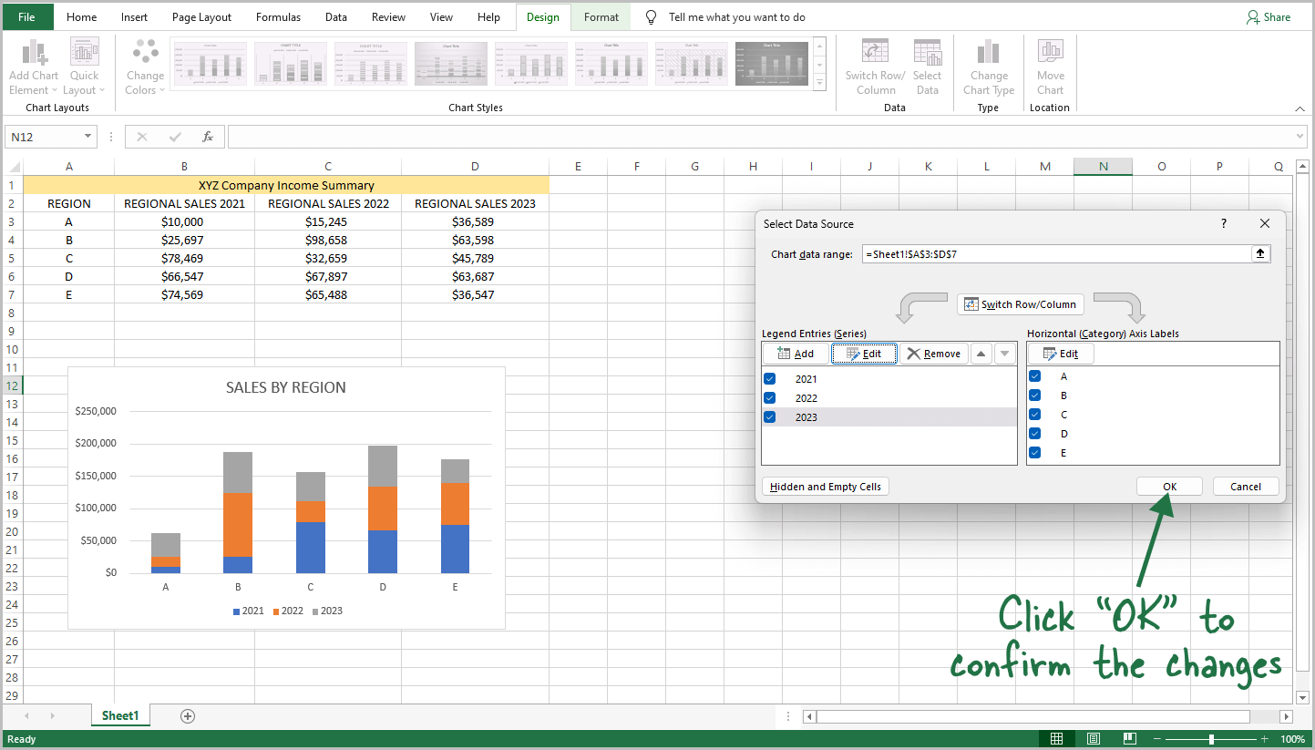
You will now see the “Select Data Source” window again.
Check whether all the legend names are correct.
Next, click on the “OK” button to confirm and save the changes.
FAQs
How do I change the legend text in Excel chart?
To change the legend text in an Excel chart, click on the chart, select “Design” from the top menu, click “Select Data,” choose the legend entry you want to modify, click “Edit,” enter the new name, and click “OK” to confirm the changes.
How do you change the name of a series in a legend in Excel?
To change the name of a series in an Excel legend, select the chart, go to “Design,” click “Select Data,” choose the legend entry, click “Edit,” replace the current name with the new one, and click “OK” to apply the change.
How to change legend text in Excel pie chart?
To change legend text in an Excel pie chart, select the chart, click “Design,” choose “Select Data,” select the legend entry, click “Edit,” change the name in the “Series name” field, and click “OK” to save the modification.
How to change legend text in Excel pivot chart?
To change legend text in an Excel pivot chart, click the chart, go to “Design,” select “Select Data,” choose the legend entry, click “Edit,” input the new name in the “Series name” field, and click “OK” to confirm the change.
Edit legend text in Excel
To edit the legend text in Excel, select the chart, click “Design,” pick “Select Data,” choose the legend entry, click “Edit,” replace the current name with the desired one, and click “OK” to finalize the editing.
Summary
Changing the legend text in Excel is a simple process that can be done in just a few steps.
Here’s how to change legend text in Excel:
- Click on the chart to select it
- Select the “Design” option from the top menu
- Click on “Select Data”
- Select a legend entry and click on “Edit”
- Enter the new name in the “Series name:” area and click “OK”
- Repeat steps 4-5 for the other legend entries
- Click “OK” on the “Select Data Source” window to confirm the changes

