Are you wondering how to freeze three or more columns in Google Sheets?
Typically, to freeze columns, you select them and navigate to View > Freeze, where you can choose to freeze either 1 or 2 columns.
But what if you need to freeze more than two columns?
Is that even possible in Google Sheets?
Yes, it certainly is!
You can easily freeze three or more columns.
This tutorial will guide you through the process, step by step.
Also read (opens in new tab):
How to Print Google Sheets Without Gridlines
How to Make a Progress Bar in Google Sheets in 4 Easy Steps
How to Highlight a Word in Google Sheets in Just 3 Easy Steps
Group Sheets in Google Sheets
How to Freeze 3 Columns in Google Sheets
1. Select the first two columns that you want to freeze
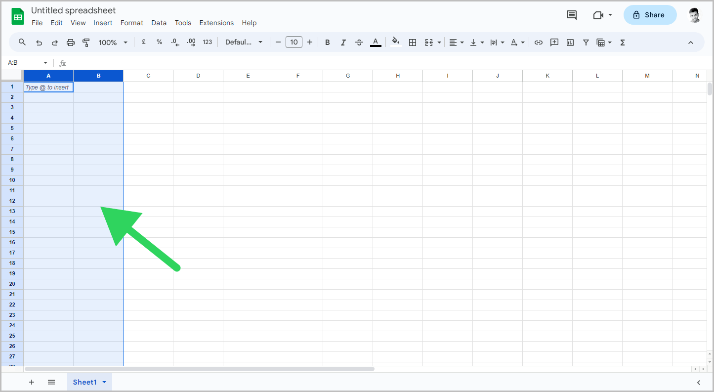
The first step is to select the first two columns you want to freeze.
For example, if you want to freeze columns A, B, and C, begin by selecting columns A and B.
Then proceed to the next step.
2. Go to View > Freeze > 2 columns
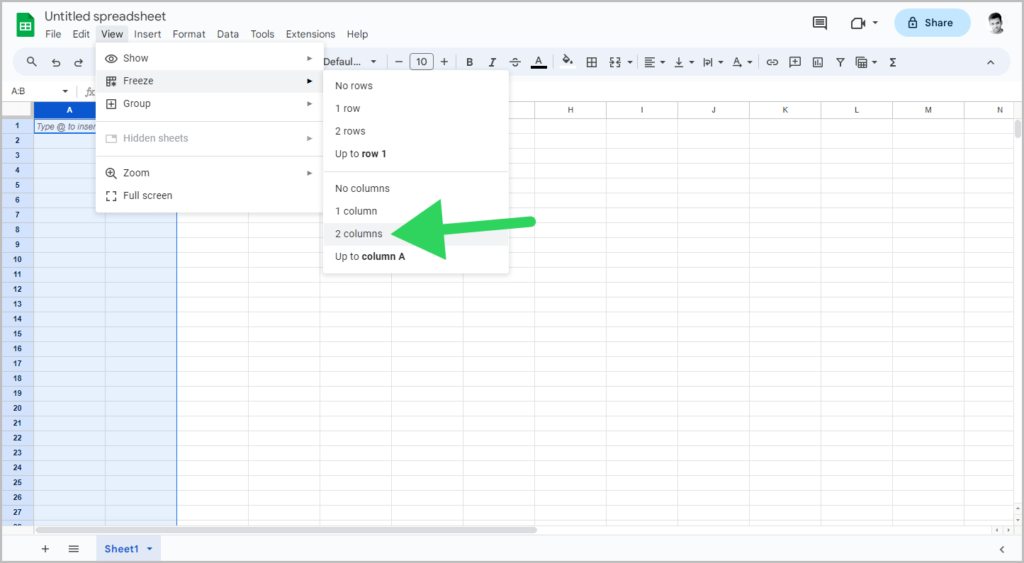
After selecting the columns, click on the “View” option from the top menu.
Then, select the “Freeze” option and finally choose the “2 columns” option from the submenu.
3. Hover your cursor over the grey vertical line until you see the hand cursor

You will now see a grey vertical line between the second and third column.
Hover your cursor over this line until it changes to a hand cursor (Refer to the screenshot above.)
4. Click and drag the line to the end of the third column
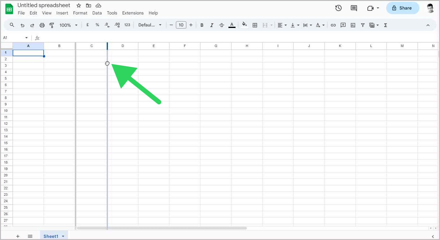
Once the cursor turns into a hand, click and drag the grey line to the end of the third column.
This action will freeze the third column.
You can also drag it to the end of any column you wish to freeze.
For instance, to freeze columns A through Z, drag the grey vertical line to the end of the Z column.
Similarly, you can freeze as many rows as needed.
To unfreeze the columns, simply navigate to View > Freeze > No columns.
Why can’t I freeze more than 2 columns in Google Sheets?
The Freeze menu doesn’t offer an option to freeze more than two columns. However, you can freeze the first two columns and then drag the grey line to the end of the column you want to freeze.
How to unfreeze columns in Google Sheets?
To unfreeze columns in Google Sheets, navigate to the “View” option in the top menu. Then, select the “Freeze” option and finally choose the “No columns” option from the submenu. This will unfreeze all previously frozen columns.
How many columns can I freeze in Google Sheets?
In Google Sheets, you can freeze as many columns as you need.
Conclusion
- Freezing columns in Google Sheets is a useful feature that allows you to keep certain data visible while scrolling through the rest of the sheet.
- The process to freeze more than two columns requires freezing the first two and then dragging the grey line to encompass the additional columns you want to freeze.
- Unfreezing columns is as simple as navigating to the “View” option in the top menu, selecting the “Freeze” option, and finally choosing the “No columns” option from the submenu.
- You can freeze as many columns as you need in Google Sheets, providing a great deal of flexibility for managing your data.

