Are you wondering how to make a progress bar in Google Sheets?
Progress bars are a useful tool for visualizing the progress of a task or project.
Fortunately, you can easily insert a progress bar in a cell using a simple formula.
In this tutorial, we will guide you through the step-by-step process of creating a progress bar in Google Sheets.
Also read: (opens in new tab)
How to Stop Google Sheets from Removing Leading Zeros
How to Highlight a Word in Google Sheets
How to Remove Underline in Google Sheets
How to Share Only One Sheet/Tab in Google Sheets
Group Sheets in Google Sheets
How to Make a Progress Bar in Google Sheets
To make a progress bar in Google Sheets, input progress data as percentages in a column, then use the formula =SPARKLINE(B2,{“charttype”,”bar”;”max”,100;”min”,0;”color1″,”green”}), and drag it down the column for multiple cells.
1. Enter your progress data as percentages in a column
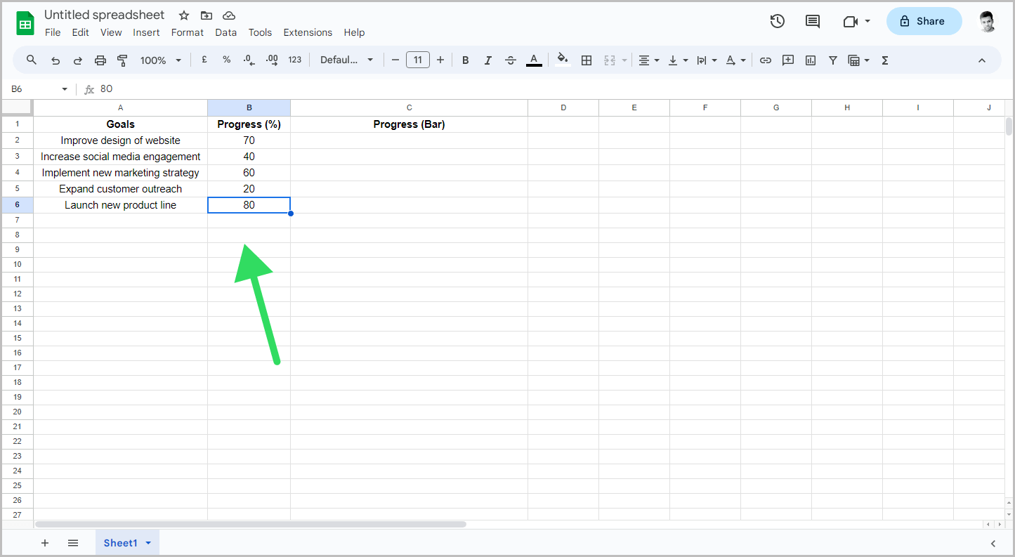
Skip this step if you already have the data ready.
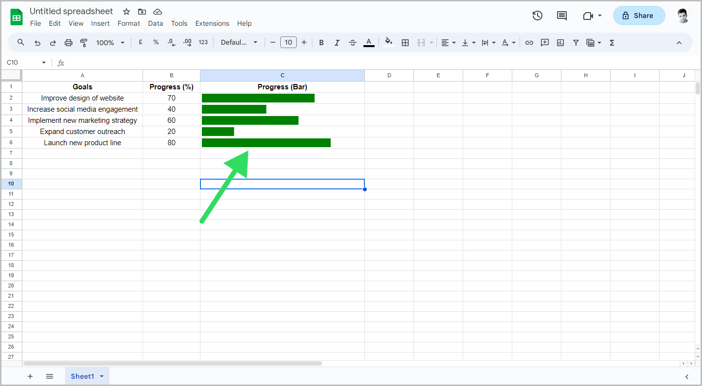
To begin, create three columns: Goals, Progress (%), and Progress Bar.
In the Goals column, list all your goals or tasks.
In the Progress column, enter the corresponding progress percentage for each task listed in the Goals column.
2. Click in the first cell of the next column
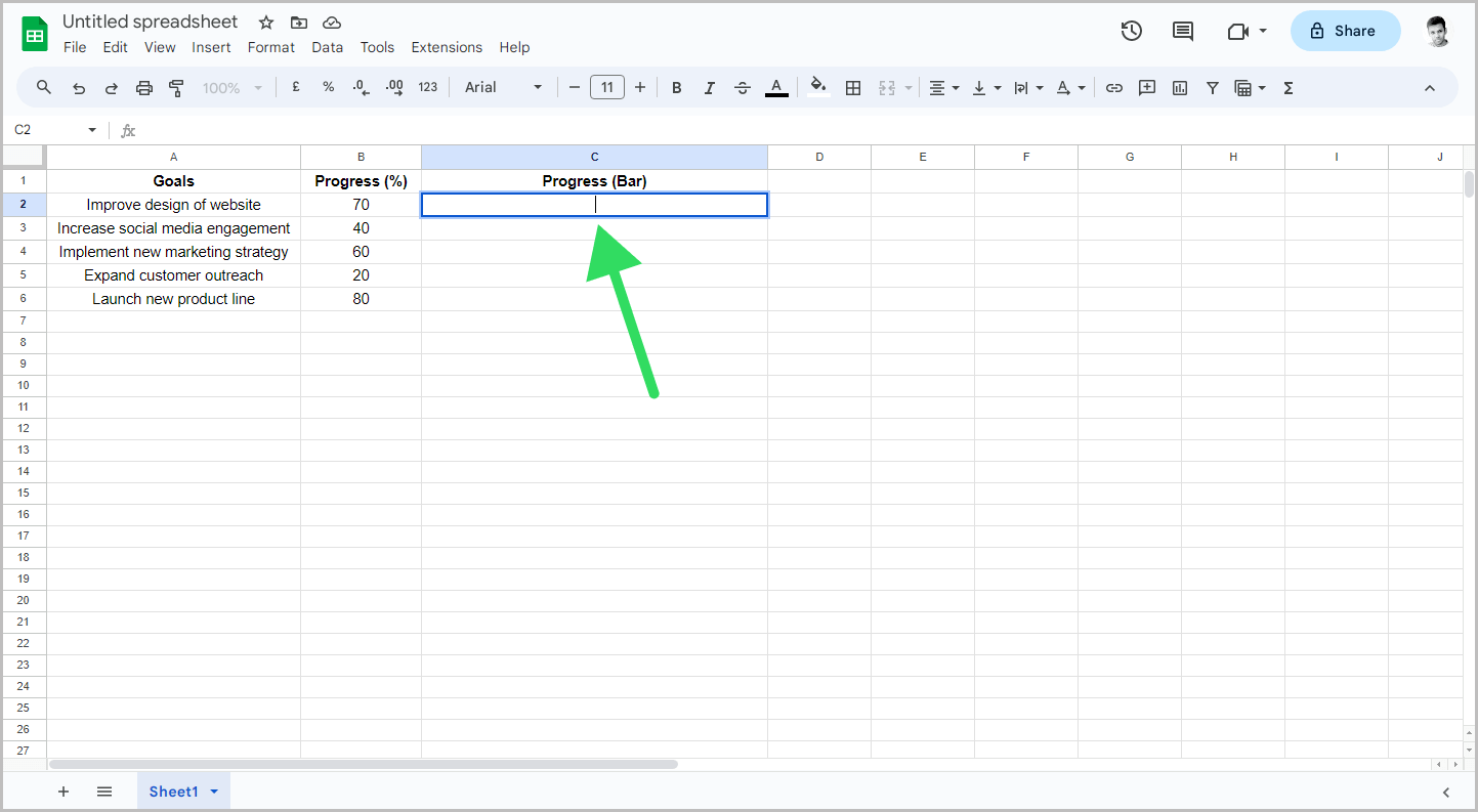
Once your data is ready, click inside the cell where you want to insert the first progress bar.
In my case, it was the first cell of the Progress Bar column or cell C2.
3. Type the given formula and press Enter
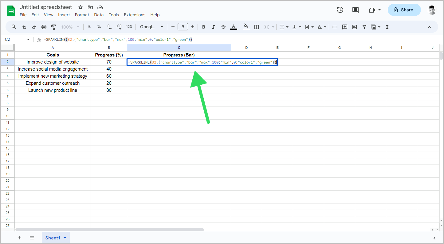
Inside the cell, enter this formula:
=SPARKLINE(B2,{"charttype","bar";"max",100;"min",0;"color1","green"})
Let’s break down the components of the formula
- B2: This represents the reference to the cell containing the data for the progress bar. The progress value is stored in cell B2. Change this value as necessary. If the first data is stored in a different cell, enter that cell number here.
- {“charttype”,”bar” ; “max”, 100 ; “min”, 0 ; “color1”, “green”}: These are the options or parameters provided to the SPARKLINE function.
- Let’s examine each of them:
a. “charttype”, “bar”: This specifies the type of chart to be created, in this case, a bar chart. It will display a simple bar representing the value in the referenced cell.
b. “max”, 100: This sets the maximum value for the progress bar. In this case, the maximum value is set to 100.
c. “min”, 0: This sets the minimum value for the progress bar. In this case, the minimum value is set to 0.
d. “color1”, “green”: This sets the color of the bar. In this example, the color is set to green. You can replace “green” with any other valid color name or code to change the color of the bar as per your preference.
After modifying the formula, press the Enter key on your keyboard.
You should then see the first progress bar.
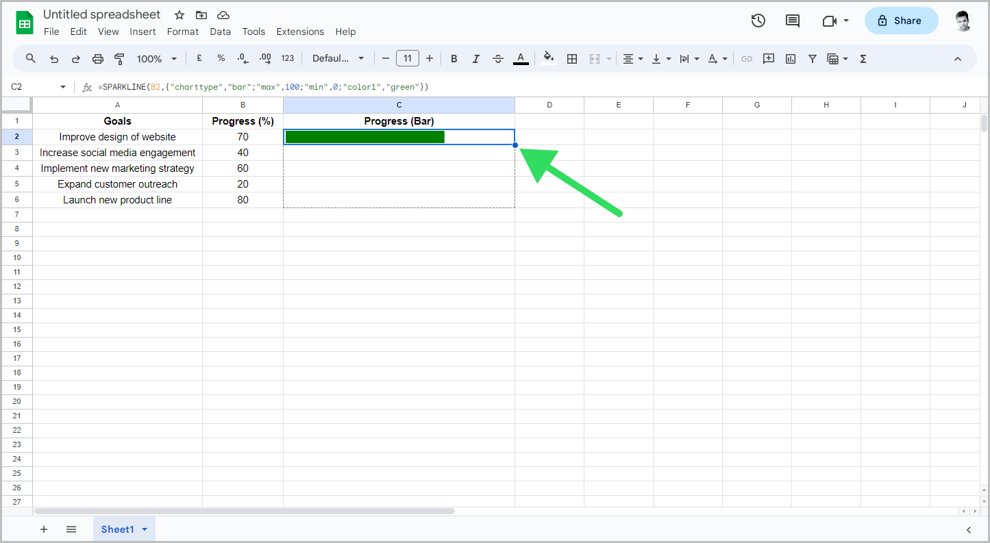
4. Drag the formula down the column to create progress bars for each cell
Now, you can enter the formula for each cell and update the cell number in the formula accordingly.
However, this can be a tedious task.
A simple workaround is to drag the formula down the column to create progress bars for each cell.
Just click inside the first progress bar that you created in the previous step.
The cell will now have a blue border with a small circle on the bottom right corner.
Click on this small circle and drag it down to apply the formula to the remaining cells.
Conclusion
- Progress bars are a visual way to track the progress of a task or project.
- Use the SPARKLINE function to create progress bars.
- Here’s how to make a progress bar in Google Sheets:
- Enter your progress data as percentages in a column.
- Click in the first cell of the next column.
- Type the formula and press Enter.
- Drag the formula down the column to create progress bars for each cell.
